Tracing Tools

Network Trace

The Network Trace tool allows the user to determine which pipes, valves or parcels will be affected if a network is interrupted within the context of water/sewer utilities. Water/Sewer network tracing starts from a selected pipe and traces to find the connected nodes and pipes that would be affected if something were to happen to the selected pipe.

For this network trace to function select the water/sewer pipe or node to perform a network trace on. Click the Network Trace button. A side pane will open displaying various options according to the type of pipe that has been selected.

Network Tracing is also now available for Fiber utilities, which incorporates powerful capabilities for the end user and becoming extremely beneficial for organizations in a modern-day context. Fiber network tracing can start with a Fiber node, Fiber Cable or Cable Route and work through the network to display desired results, based on the trace option selected. For this network trace to function select the Fiber node to perform a network trace on.

Note: Different trace options will appear for water, sewer and fiber network traces.

To change the Selected results to display after a trace was run select the same water or sewer object/s from the map and select the Network Trace function from the enlighten toolbar. Select the desired results to display from the Selected results to display options and run the trace again.

Once a network trace has been run you can switch between water and sewer traces by selecting either water or sewer objects without selecting the Network Trace function again. Alternatively refreshing the map, without making any selections, would inevitably bring up the Fiber network trace pane. The various water, sewer and fiber trace options will be discussed below:

Water Pipe Network Tracing

If a water pipe is selected the user can choose to perform either a:

Pre Calculated Trace: Switch on/off the availability of using pre-calculated shut-off block trace result.
System Trace: Only the selected section of the network will be subjected to a network trace.
Full Trace: All the sections of the network that do not have any other source of supply will be selected when a full trace is conducted.
Part Trace: The trace will stop when the closed or nearest valve has been reached. The trace will traverse the network in all directions from a given point of failure/leak and calculate the valves that will define a Shut Off block.

Before running the trace, the user can choose which layers will be displayed in the Water Pipe Trace Results window. If the service connection table contains both parcel GID and property GID data, the user can choose to see either the affected parcels or the affected properties in the result window:

Affected Water Pipes
Affected Pipe Volume
Affected Valves
Affected Service Connections
Affected Parcels or Properties

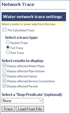
Fig: Water Network Trace

After the initial water pipe trace has been conducted an option appears that is called Trace Through. The Trace Through option should be used if a valve cannot be physically closed for any reason (rusted/covered).

The user can select the offending valve on the map and trace through that valve. This option will re-calculate and extend the trace to exclude that valve from the network trace. To stop a trace prematurely you can select a ‘Stop Predicate’.

Sewer Pipe Network Tracing

The Sewer Network Tracing function provides the ability to perform different types of trace from a graphically selected sewer pipe. The user can choose to perform an upstream or downstream trace.

Upstream Trace: All the pipes and parcels which have service connections connected to the pipes that flow to the selected pipe will be found.
Downstream Trace: All the pipes and parcels which have service connections connected to the pipes that flow from the selected pipe will be found.

The user defines what layers will be displayed in the Sewer Pipe Trace Results by checking or unchecking the display boxes:

Affected Sewer Pipes
Affected Pipe Volume
Affected Service Connections
Affected Parcels or Properties

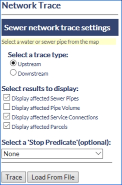
Fig: Sewer Network Trace

If the sewer service connection table contains both parcel GID and property GID data, the user can choose to see either the affected parcels or the affected properties in the result window. To stop a trace prematurely you can select a ‘Stop Predicate’.

Stop Predicates

The enlighten administrator has the ability to define Stop Predicates in the administration section of enlighten for sewer and water network traces.

Stop predicates are described as a condition at which the trace is forced to terminate prematurely if a certain condition is satisfied during the trace. In the instance of enlighten, a stop predicate may be an access point of a particular type, a change of pipe diameter, or a specific valve type, etc. The purpose of stop predicates is to find information using network trace functionality, without performing a standard network trace, i.e. when a stop predicate is selected, the valves and water sources etc. will be ignored and the stop predicate condition will be searched for.

The Trace direction is only triggered once the number of max pipes is set and will run bi-directional traces. If the Maximum number of pipes is set to NULL then the trace will run with default value of 250 pipes, and the resultant trace will still run bi-directionally. If the Trace number of pipes is entered, then the other parameters are not necessarily ignored since the trace result depend on the data on the map and on the parameter values entered in the Stop Predicate.

By default, the stop predicate condition for a network trace is None, meaning that no stop predicate will be used in the trace.

To define a stop predicate the user simply selects a predefined Stop Predicate condition from the drop-down list and sets the condition requirements.

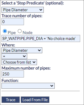
Note: When a stop predicate is selected, the default network trace behavior is overwritten.

Fig: Stop Predicate Options

When the user selects either a Pipe or Node as a Stop Predicate, the system dynamically updates the referenced table and generates the SQL with the first column of the table being highlighted in the where clause. If the new column being specified has no lookup assigned to it, then it will revert to a free text input box.

Manually entering a value within double quotes will return a SQL error as the system is not configured to tolerate it. Using the keyword “SAME” or “same” would default the variable to the selection from the database column bein3g referenced.

If a numeric value is entered in the SQL dialog, then it is not validated if a lookup value list is displayed. Ordinarily one would select the value in the lookup table, and it would be automatically pasted into the SQL dialog. Manually entering a value in the SQL dialog would be done if for some reason the lookup table was not populated with that value.

A Stop Predicate can be applied to a Water or Sewer Network Trace and can be defined for pipes or nodes.

Trace number of pipes: The number defined in this section defines the number of pipes to trace through if the predicate condition is not met. For a water trace this is the number of pipes in both directions, and for a sewer pipe trace it is the number of pipes in a single direction.
Maximum number of pipes: This field is the highest priority in the stop predicate. When a number is entered in this field it disables every other predicate condition. For a water trace, this is the number of pipes in both directions and for sewer pipes trace it is the number of pipes in a single direction.

A Function lookup has also been added to qualify the predicate condition. Some Oracle functions have been made available via the lookup table EN_TRACE_FUNCTIONS:

Left Trim: Removes all leading spaces.
Right Trim: Removes all trailing spaces.
Lower Case: Removes all trailing spaces.
Upper Case: Removes all trailing spaces.
To Number: Removes all trailing spaces.
NT_CONV_VAR2NUM: Removes all trailing spaces.

To define a stop predicate the user simply selects a Stop Predicate condition from the drop-down list and sets the condition requirements.

Network Trace Results

After performing a Network Trace, the user can choose to view or save the information retrieved. A tabular output of the network trace results can be accessed by selecting the Show Report link on the Network Trace Result dialog. The results are then shown in the standard enlighten Show Info. The columns displayed on the Show Info pane are pre-defined by the enlighten administrator.

Network Trace results are saved using the ‘Shut Off Reporting’ or ‘Selections’ functionality

Load From File

If a pipe selection was saved to a file, this can be retrieved and traced on by selecting the Load from File option. Pre-loading map selections before running a trace will override the trace package. The selections need therefore to contain Pipes and Nodes for Water trace and Pipes only for Sewer. Other objects included in the selection will be ignored.

Note: Non-Return Valves (also called Check Valves) are processed during network tracing in the following manner. When the tracing process reaches such a node through a pipe, it checks if the node rests at the start point of the coming pipe. This is true when the START_NODE of the coming pipe has a value equal to the NODE_ID of the node. In such a case the tracing goes through the node as if it does not exist. Otherwise, when the END_NODE of the coming pipe is equal to the NODE_ID of the node, the tracing stops at that node.

Sewer Pipe Trace Example

To conduct a sewer pipe trace, first select a sewer pipe then click the Network Trace icon from the Advanced Toolbar. In the Network Trace pane the following prompts can be used to conduct a sewer pipe trace.

To start a trace:

Select the direction of the trace Upstream or Downstream.
Select the layers to be displayed in the results.
Select whether to have the pipe volume displayed in the results.
Alternatively, select a Stop Predicate (set up by the administrator).

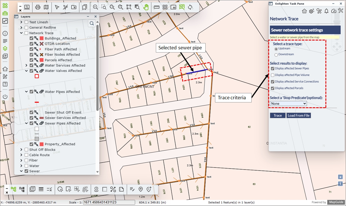
Fig: Sewer Pipe Network Trace Dialog Box
The Network Trace results are displayed on the map and the number of affected features is displayed in the Network Trace pane.

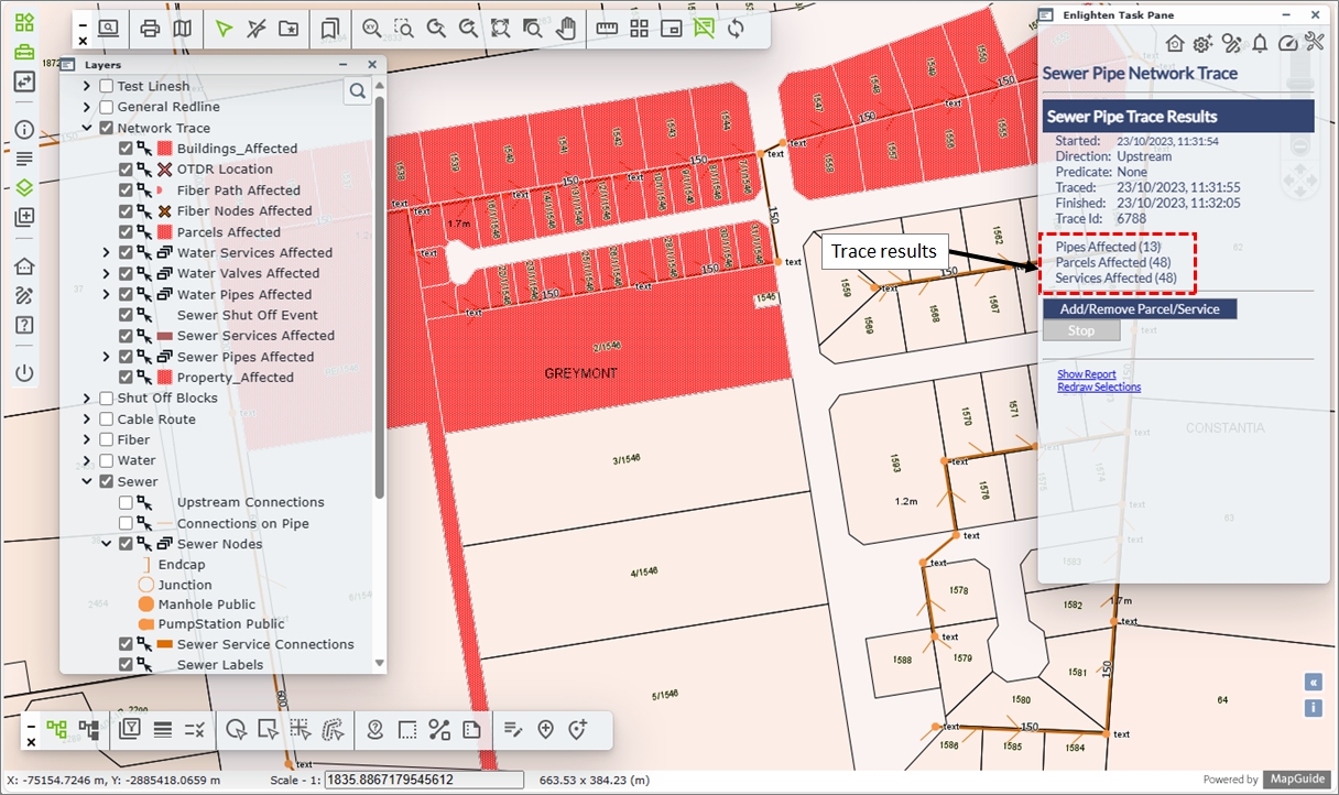
Fig: Results from Sewer Pipe Network Trace Analysis

The map is zoomed to the extent of the trace results and the Affected Pipes and Parcels are highlighted and selected. The number of Pipes Affected and/or Service Connections and/or Properties/Parcels Affected is shown as part of the Sewer Pipe Trace Results.

The Add/Remove Parcel/Service option provides the ability to add or remove one or more objects from the trace selection. The user can continue adding or removing objects to/from the trace selection until the Stop option is clicked. If the selection set is lost, it can be retrieved by selecting the Redraw Selections option.

Further information pertaining to Adding/Removing Parcels/Properties/Buildings can be found within the enlighten Administrators guide under the Configure Settings section > Network Trace > Service Connection Linking.

Further reporting is available by clicking on the Show Report link. To save the results please refer to ‘Shut Off’ reporting or ‘Selections’

Water Pipe Trace Example

If a water pipe has been selected, the Water Network Trace Settings set up side pane will appear. If a pipe selection was saved to a file, this can be retrieved and traced on by selecting the Load from File option.

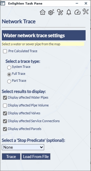
Fig: Water Pipe Network Trace Dialog Box

To start a trace:

Choose to do a Pre Calculated, System Trace, Full Trace or Part Trace. The Full Trace is the default and will automatically include in the trace all the sections of the Network with no other source of supply, Part Trace will isolate the network to the closest valves in each direction (the trace will stop when the nearest node defined as valve has been reached.
Select the required results (Affected Water Pipes and/or Affected Valves and/or Affected Service Connections and/or Affected Properties or Parcels).
Select whether to have the pipe volume displayed in the results.
If a Stop Predicate is selected, this will override the tracing package.
The Network Trace results are displayed on the map and the Water Pipe Trace Results window will appear as shown below.

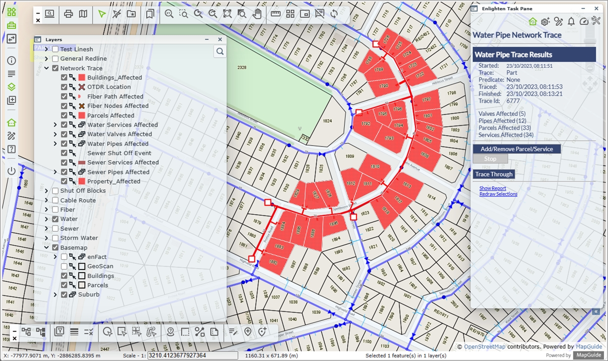
Fig: Results from Water Pipe Network Trace Analysis

The map will be zoomed to the extent of the trace results and the affected objects highlighted along with the pipe volume if that option was selected.

The Add/Remove Parcel/Service option provides the ability to remove one or more objects from the trace selection. The user can continue adding or removing objects to/from the trace selection until the Stop option is clicked. If the selection set is lost, it can be retrieved by selecting the Redraw Selections option.

Trace Through functionality is only available in water network trace and allows continuing the trace through a selected valve to the next one. This option is used, for example, when a valve cannot be closed or is broken, and the operator needs to identify the next nearest one.

The process for tracing through a valve is:

From the Water Trace Results dialog, click on the Trace Through button.
Click on an Affected Valve on the map. These are indicated as red squares on the map.

If an affected valve is not selected, a message dialog will be displayed saying Please select an Affected Valve to trace through.

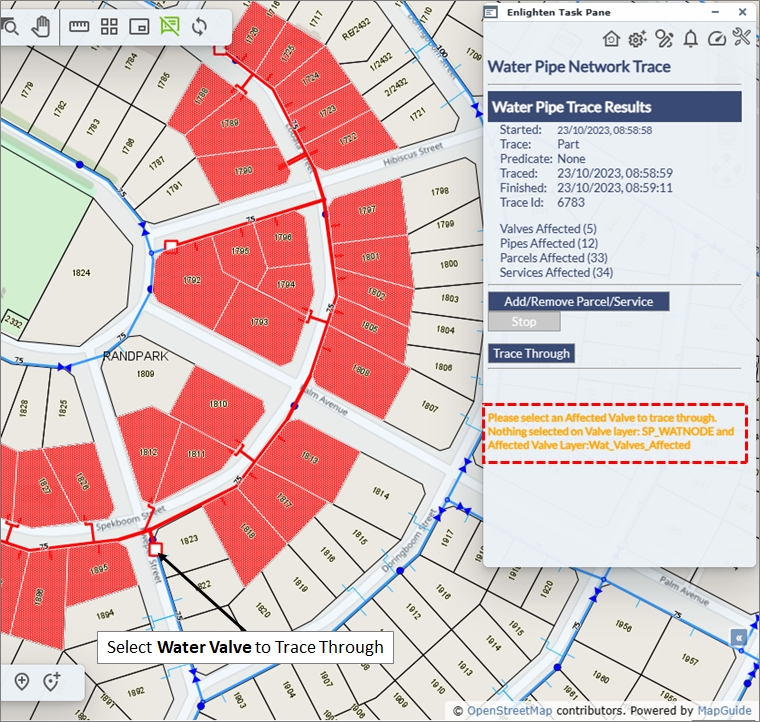
Fig: Results from Water Pipe Network Trace Through

When an Affected Valve is selected, the program will perform the re-trace and then display the new result set on the map. The Water Pipe Trace Results in the right pane is updated with the number of Valves, Pipes, Parcels, and Services affected. The Trace Through can be repeated until the user is satisfied with the extent of the trace. For each trace, the Water Pipe Trace Results in the right pane is updated.

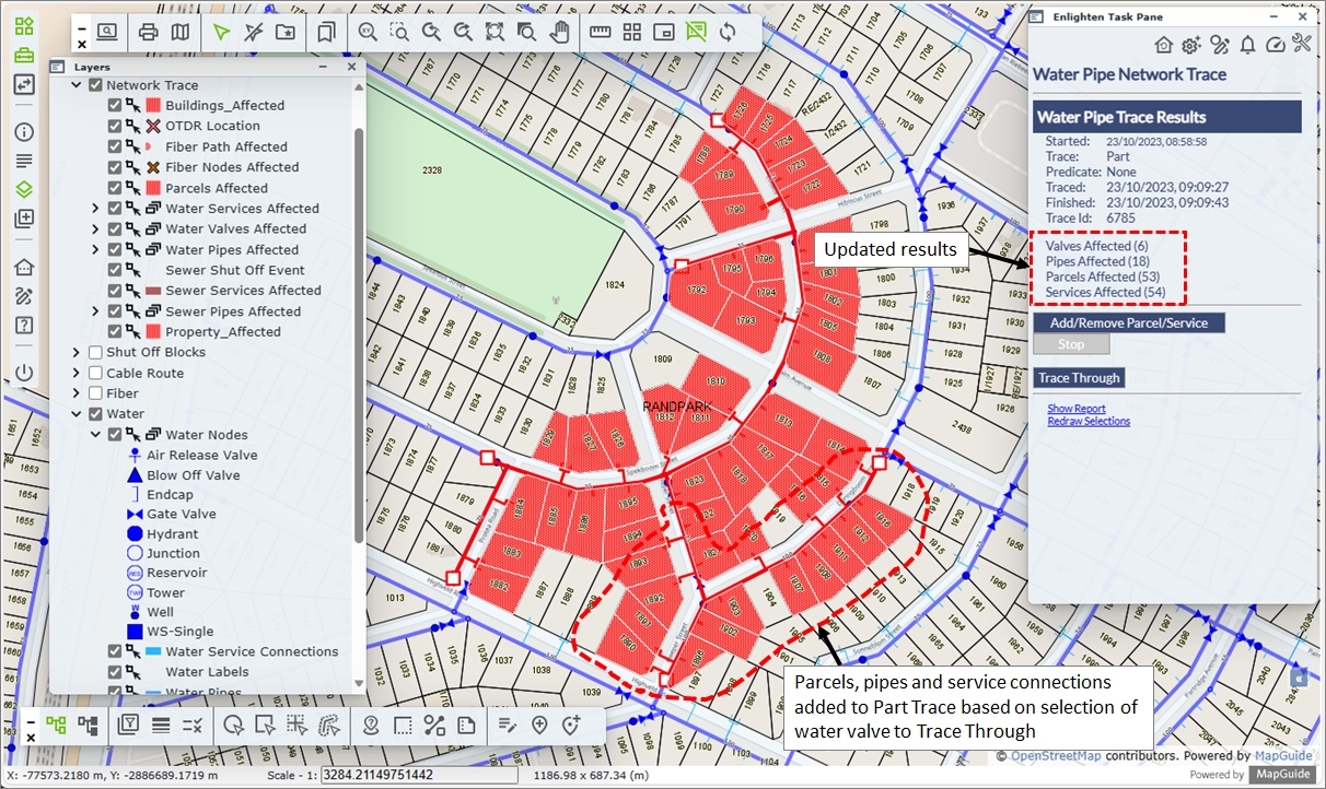
Fig: Results from a secondary Water Pipe Network Trace Through

Water Pipe Stop Predicate Example

If a water pipe has been selected, the Water Network Trace Settings set up side pane will appear. If the Stop Predicate option is selected, the parameters are displayed in the side pane for user configuration. For this example, the following Stop Predicate parameters have been set.

Set the Stop Predicate by selecting Pipe Diameter from the drop-down list.
Set the Trace number of pipes to trace 3 water pipes.
The Where Clause is partially set based on the the Pipe Diameter selection above, however you will need to set the Pipe Diameter criteria, for example, select the greater than operator > , and select a pipe diameter from the available drop-down list, for example 140.
Set the Maximum number of pipes to only trace 5 pipes, remembering this field is the highest priority in the stop predicate.

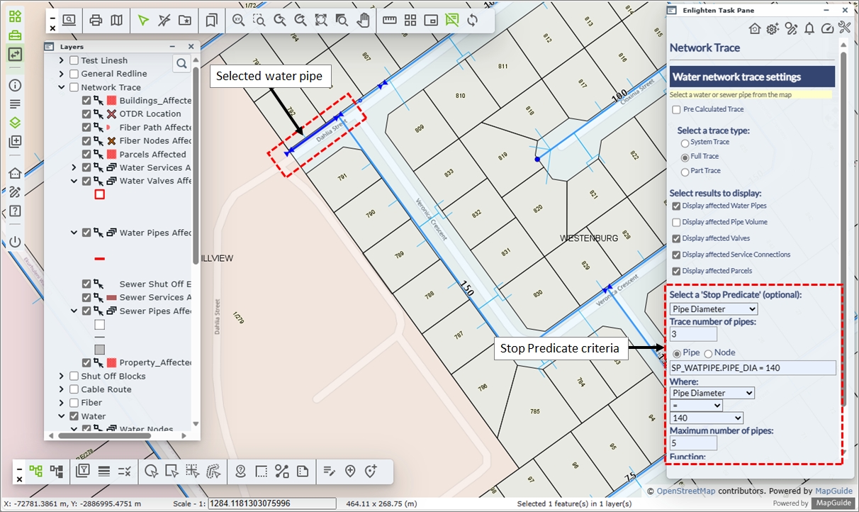
Fig: Water Pipe Network Trace Dialog Box with Stop Predicate parameters

The results of the Water Pipe trace after applying the Stop Predicate are displayed in the Water Pipe Trace Results section on the side pane, and the affected Parcels, Pipes, Service Connections and Valves (based on the Selected Results to display) are all highlighted in the map.

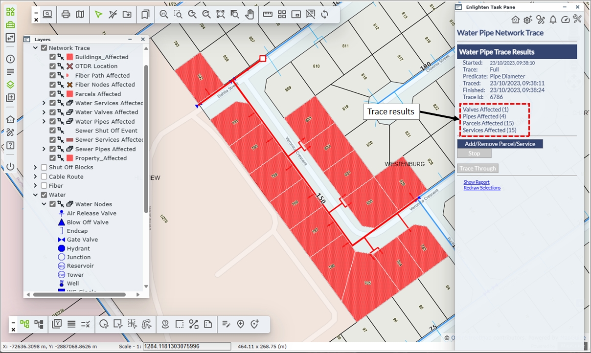
Fig: Water Pipe Trace Results after applying the Stop Predicate

By selecting the Show Report option, the affected parcels, water pipes and service connections can be viewed in the Show Info pane if these forms have been defined. If on the Show Info pane the Map Layer count is displayed in black, it indicates there is an Advanced Form defined, whereas if the objects are displayed in grey, no form has been defined.

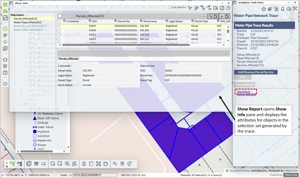
Fig: View Water Pipe Trace Results in Advanced Forms

The Affected Parcel records displayed in the Show Info pane can be exported to a .csv file for reporting purposes by selecting the Export CSV button on the Show Info pane.

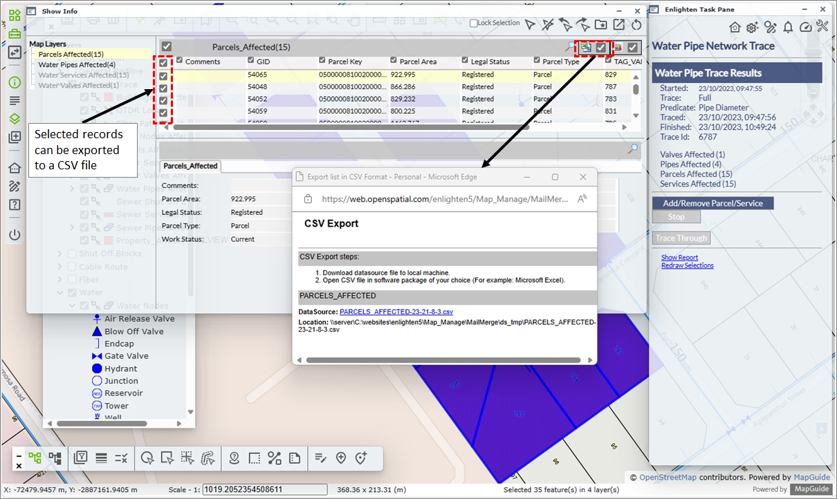
Fig: Affected Parcel records displayed in the Show Info pane can be exported to a csv file

The exported .csv file can be imported into Excel and saved as a spreadsheet.

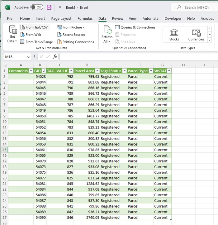
Fig: Import csv file into Excel

Network Trace (Manual Mode)

When the user runs a Network Trace in Manual Mode, then the system is manipulated into returning the results only of what the user manually selected before running the trace. Network trace can be run in Manual Mode, for both the Water and Sewer utilities.

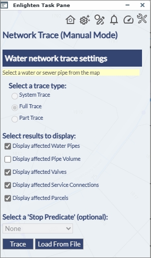
Fig: Network Trace Manual Mode

To start a Network Trace in manual mode:

Select the relevant Pipes/Valves and Property/Building/Parcels, which is desired to be outputted. (selecting 2 pipes and a valve also triggers manual mode).
Click on the Network Trace Icon.
Select whether to have the pipe volume displayed in the results.
If a Stop Predicate is selected, this will override the tracing package.
The Network Trace results are displayed on the map and the Water Pipe Trace Results windows will appear as shown below. These results will be the initial Pipes/Valves the user selected prior to running the Trace.

Note: When conducting a Network Trace in Manual Mode then the option to define the Trace type is greyed out.

Fiber Network Tracing

The Fiber Network Tracing function provides the ability to perform different types of traces from a Fiber selection made on the map. As long as fiber layers have been configured in the Network Trace Admin page, having nothing selected on the map will bring up the common route trace.

The various Fiber Network Trace options are:

Optical Time Distance Reflectonomy (OTDR): Select a relevant Fiber Node and then the Route > Cable > Tube > Strand carrying a service, enter in a distance and then the system should highlight the associated Route and Path. Important attribute information is also displayed on the screen of the map view, near the associated feature and on the right hand side task pane.
Break Trace: Select a Fiber Cable / Cable / Tube / Strand and once a trace is done, the route and path is highlighted, and activates an advanced form. On this form important information pertaining to services attached to the strand are displayed.
Common Route Trace: This trace selects a commonality between two cable routes, an overlap between the both. As with the Break, trace, the Common Route Trace also activates an advanced form.

Optical Time Distance Reflectonomy (OTDR) Trace

The OTDR trace provides enlighten users the ability to locate the point along a fiber path where a significant event or anomaly has occurred. The user must have performed a physical OTDR trace to characterize the optical fiber utilizing appropriate instrumentation and provide a distance where the event or anomaly occurs. The user must select the source node that the OTDR instrumentation has been utilized. The result of the OTDR trace in the enlighten application will show the physical location of the selected interruption with consideration of slack loops and vertical distances. The interruption point is provided within a given tolerance.

To start an OTDR Trace:

Select a Fiber Room or Fiber Joint node from the map.
Select the Network Trace icon on the Advanced Toolbar.
The trace defaults to the OTDR trace option if a Fiber Room or Fiber Joint node is selected.
The Fiber Network Trace task pane is auto-populated with the connecting Cable Routes, Cables, Tubes and Strands for the selected node.
Input the trace distance required, or accept the default of 10m.
Select the Fiber Strand containing the service by expanding and selecting the expansion boxes from Route level down through the Cable and Tube level and select the desired Strand by ticking the check-box adjacent to the desired Strand.

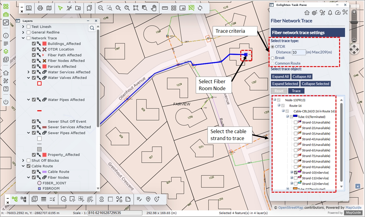
Fig: OTDR Node Selection
Once the required Strand is selected, click on the Trace button.
The OTDR Fiber Network Trace results are displayed in the Fiber Network Trace task pane.

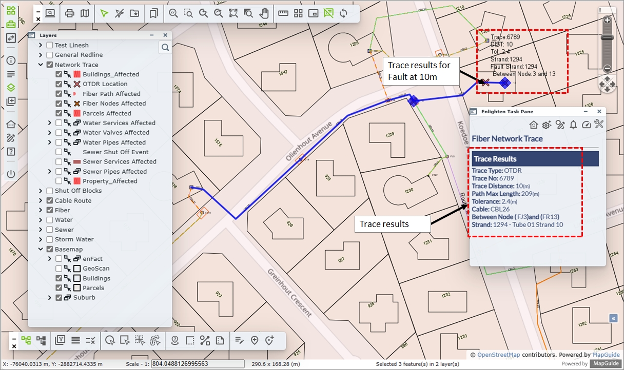
Fig: OTDR Trace Results
Selecting the option Zoom to Path option will zoom the map to a scale of 1:1000 and display the Fiber Path at the center of the screen.
Selecting the option Zoom to Fault option will zoom the map to a scale of 1:1000 and display the Fiber Fault at the center of the screen.

Break Trace

The Break Trace indicates to enlighten users the start point of a fiber cable, the end point and also what services are running on the fiber cable. By using this trace option, the user would be required to expand the tube of interest, and thereafter expand the actual strand. The user would then be able to see the relevant service which is attached to the fiber strand. Once the trace has been successfully completed, then the advanced form would pop, with important information pertaining to the service attached to the fiber strand.

To start a Break Trace:

Select a Fiber Cable from the map.
Select the Network Trace Icon from the toolbar.
The Fiber Network Trace task pane is auto-populated with the selected Cable Tubes and Strands. Select the relevant Cable > Tube > Strand containing the service. This selection can be at Cable level, Tube level or at Strand level.

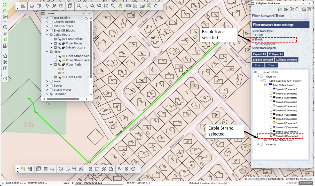
Fig: Break Trace Criteria
Click on the Trace button.
The Show Info Pane is opened, containing associated results.

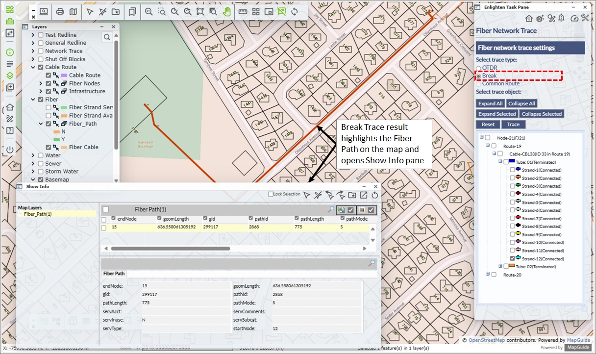
Fig: Break Trace Result

Common Route Trace

The Common Route trace enables enlighten users to identify the cables that interact with a given service identifier. This enables the user to identify the cables of interest when analyzing an event that has occurred potentially reducing the time required to resolve network impact.

To start a Common Route Trace:

Select the Network Trace icon from the toolbar.
Enter in the relevant Service IDs, for example, SAC2035 and SAC2036.

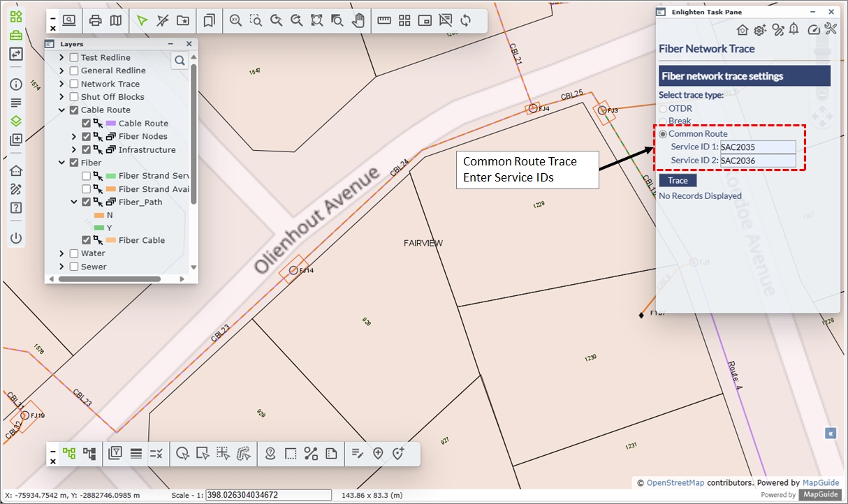
Fig: Common Route Trace Criteria
Click on the Trace button.
The Show Info pane is opened displaying the attribute values for the entered Cable Route.

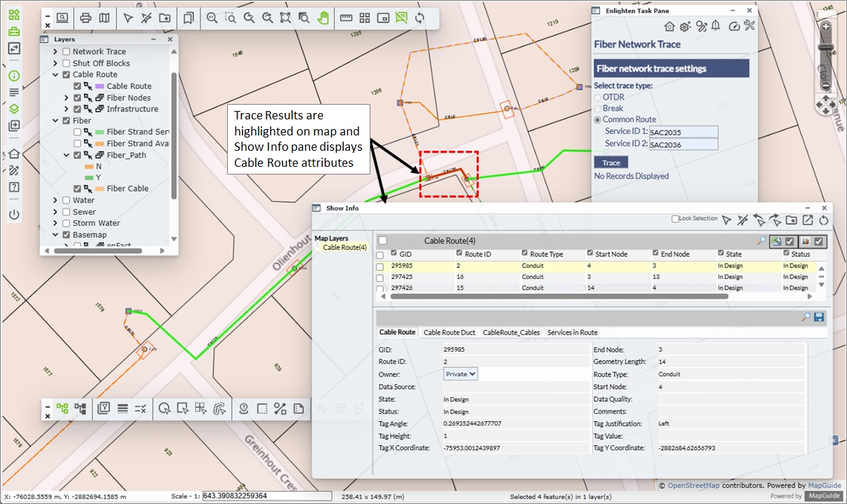
Fig: Common Route Trace Results

Network Trace Error Messages

If enlighten does not have any layers configured for network traces, the following message will be displayed if the Network Trace icon is selected.

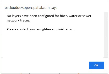
Fig: Error Message when no Network Trace Layers are configured

If enlighten only has Fiber layers configured for network traces, the following message will be displayed if the Network Trace icon is selected and no objects, or the incorrect objects are selected in the map.

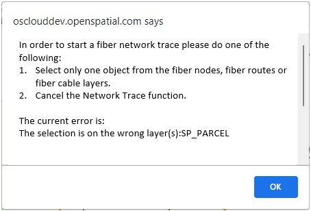
Fig: Error Message when only Fiber Network Trace Layers are configured

If enlighten only has Sewer/Water layers configured for network traces, the following message will be displayed if the Network Trace icon is selected and no objects, or the incorrect objects are selected in the map.

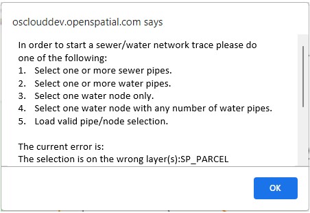
Fig: Error Message when only Sewer/Water Network Trace Layers are configured

If enlighten has Fiber and Sewer/Water layers configured for network traces, the following message will be displayed if the Network Trace icon is selected and no objects, or the incorrect objects are selected in the map.

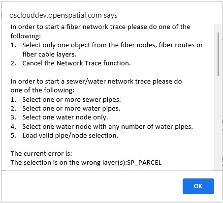
Fig: Error Message when Fiber and Sewer/Water Network Trace Layers are configured

Shut Off Report

The Shut Off reporting tool is located on the Advanced toolbar.

Two options are available in the Shut off reports tool you can either save a new report or update an existing report. To open save report click the reports tool with features selected in the map. To enter the update report tool there must be nothing selected on the map.

When the ShutOff function is being executed on a Water pipe and the user clicks on a Water pipe in the map, then the task pane will change to reflect the relevant associated map feature. The consistent fields amongst these two features will maintain the user inputted data, however some fields will still need to be filled in.

Save Report

To save a new report you must first have at least one service connection selected on the map. Save report is often used after selecting multiple features using ‘Network Trace’ or other spatial functions.

The following information must be entered in the Save Report window:

The Report Type which in this case is Shut Off.
If the event is Planned or Unplanned.
The Event Type or Cause what is the problem with the pipe? The options include burst, hydrant, leak, other, service and valve.
The Service Request Number that is a unique numerical identifier for the event.
The Event Time the event occurred (e.g. 12:00 pm)
The Event Date the event occurred (DD/MM/YYYY), which can be selected from a date picker.
The Duration of the event (whole minutes).
The Event Description for the event.
The Water Category type abandoned, portable, raw, reclaim or all if the network does not have a specific category value.
Additional Remarks where further comments can be made.

The user is required to enter in a Service Request Number before generating the report. If the user attempts to run a Shut Off Report without a Service Request Number assigned, the system will flag an error. The error message displayed will be: Shut-Off not saved. Request Number cannot be null.

The user would also have to ensure that a unique Service Request Number is specified. If the user enters an existing Service Request Number to be saved when generating a new report then the following error message will be returned: Shut-Off not saved. Record already exists with the same service request: X (X being the actual service request number).

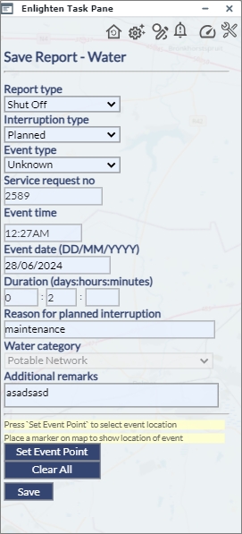
Fig: Save Shut Off Report Side Pane

After entering the required information, it is optional to Set a Event Point. To do this, click on the Create Event Point button and then the cursor will change. The operator then must click on the map on or near a pipe or node. When a point on the map has been clicked a pre-set symbol (created by the enlighten administrator) will appear on the map to mark the spot.

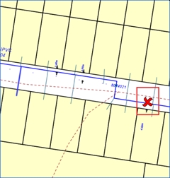
Note: The X marker is a temporary object on the map and will not reappear if the window were subsequently refreshed.

Fig: Event Point

When the user hits Create Event Point, then the following message will be displayed:

"Processing. Please Wait".

Thereafter Event was saved to the database will appear on the bottom of the Save Report pane.

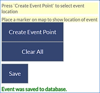
Note: The job number is what you will be able to see when you select a job in the update reports section.

Fig: Event Saved to Database

If colored parcels have been configured by your enlighten administrator they can be viewed by clicking the refresh button on the map toolbar.

Update Report

To enter the Update Report side pane, click on Shut Off Reports without anything selected on the map.

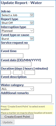
Fig: Update Report Side Pane

Note: If additional report types and event types are required then the user should create those within the Unknown type.

The details previously saved can be selected using the drop-down list in the Job No section. The jobs will be displayed by Job No in ascending order.

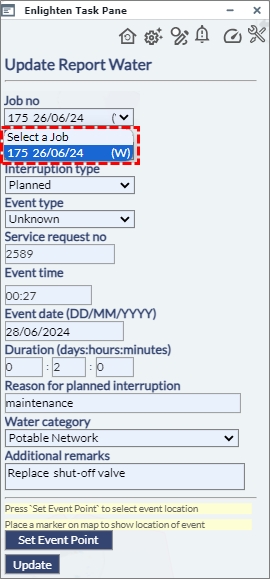
Fig: Saved Jobs

Once a job is selected, the form will automatically populate, and the map will zoom to the saved features.

If the details originally entered were not correct or have changed, they can be edited. To do this select the desired job, make the changes and click on the Update button.

Please contact the enlighten administrator for instructions of how to retrieve the saved event details. These can be displayed in a Shut Off event layer or extracted from the database in a tabular format.

Shut Off Report in Edit Mode

If nothing is selected on the map and the user clicks on the Shut off function, then the Update Report pane will be loaded (same as updating an existing job). This mode allows the user to update a report which has already been saved. If the shutoff is planned then it is updated later when the actual effects are known such as parcels added / removed and actual time taken.

enMerge

The enMerge tool allows the user to merge together the network trace, shut off report and plotting functions leaving the plot engine to handle the production of mail-merge letters. If you click on the enMerge tool with no selections on the map the following window will appear. Three workflows are available to the user.

Shut Off Report with Network Trace

The workflow is activated when a sewer/water pipe is selected on the map and the user wishes to do a network trace, Shut Off and an optional plot.

Shut Off Report

The workflow is activated when a sewer/water service connection is selected on the map. The user is presented with the choice for an optional plot.

Pre-filled Shut Off Jobs

Use this workflow to open a future Shut Off job, whose details have already been filled. The user has the choice to plot the Shut Off job if needed.

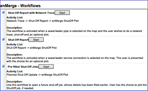
Fig: enMerge Work Flows

Workflow 1 Shut Off Report with Network Trace

Running a network trace requires an eligible pipe to be pre-selected on the map. Click on the enMerge tool and select Shut Off Report with Network Trace. When the network trace is finished and its results are selected on the map as illustrated below, enMerge will immediately invoke the second workflow Generating a new Shut Off report. For more information see ‘Network Trace’.

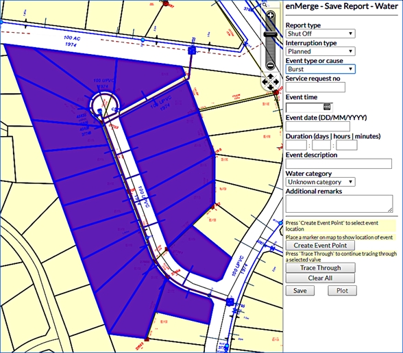
Fig: Trace Workflow Example

Workflow 2 Generate a New Shut Off Report

Creating a new Shut Off requires as a minimum that service connections are selected on the map. This is satisfied if a trace was run previously or if the user had manually performed the selections. After the form is filled in and saved (refer to the illustration below) the Plot button (which should now be enabled) can optionally be clicked to generate a plot which is displayed in its own window in a PDF format. The user can then save the plot information. For more information see ‘Shut Off Report’.

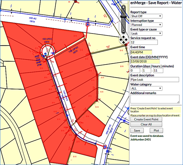
Fig: Shut Off Workflow Saved and Ready to Plot

Workflow 3 Choose a Pre-filled Shut Off Report

An alternative to workflows 1 or 2 is to have no selections on the map. The shut off form will include a new lookup to allow selection of a previously saved job (or event) as illustrated below. When you choose a saved job, the map will zoom to the saved features and the form will auto-populate. Any details can be changed once you have selected a job, including the event point. Plotting can then proceed as per work flow 2 above. For more information see ‘Shut Off Report’.

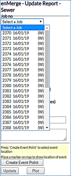
Fig: Pre-Filled Shut Off Selection and Update

Workflow 4 enMerge Plot

Once you have your report information saved and ready to use you can select to plot. Plots are configured by your enlighten administrator and vary between organizations. Please see ‘enPlot’ for more information about plotting options.

Integration Tools

The Integration tool available on the Advanced Toolbar allows third-party applications to be accessed from within enlighten. The form or application that is launched is specific for each integration, therefore further details will be provided by your enlighten Administrator.

Only users who have the permissions for the Integrations function assigned to them will have access to the Integrations icon on the Advanced Toolbar. When selected, the Integration Manager pane is opened where a list of configured application integrations are displayed in the Application list. The user must select a single application from this list and the Selections section is updated to display the Layer or Function configured for the integration application type selected. Once the Selection is completed, the user must select the Proceed button to display the relative configured integration information on a separate text screen.

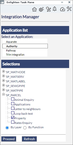
Fig: Integrations Pane displaying various application integrations.

In terms of initial enlightensetup, the integration utility does not create any integration packages. The Integration function in the Admin View provides the enlighten administrator with the tools to maintain the integration packages and their associated functions to third-party applications.

The Integrations module, only accessible to users with Administrator privileges via the Admin View, allows for registering and maintaining any third-party applications that can be integrated with enlighten. We suggest that any customer requiring integration to an external application contact out support team for assistance at Open Spatial Support.

Spatial Tools

The Spatial Function tools allow the user to detect spatial interactions between map objects as well as saving and loading spatial selections.

Drill Down Selection

The Drill Down Selection tool , located on the Advanced toolbar, prompts the user to pick a point on the map, which in turn applies the Point Buffer distance defined in the POINT_SEL_BUFFER and selects all map feature objects falling within the buffer distance. The Show Info pane is opened and populates the Tree, List and Detail views with the associated layer and attribute information for the map feature object/s selected on the map.

Nearest Neighbor

The Nearest Neighbor tool , located on the Advanced toolbar, allows the user to identify a set number of neighboring objects within a set distance of a selected map feature. To activate the Nearest Neighbor function, first, select a map feature or multiple features on the map window and then click the Nearest Neighbors button. A side pane on the right-hand side of the screen will prompt for the following information:

The target layer to perform the Nearest Neighbor search on.
The maximum distance to the selected object.
All distance sets unlimited distance (number limit applies).
The maximum number of objects to be retrieved.
All number sets an unlimited number (distance limit applies).
After typing in the required information, click on Show. The features matching the selected criteria will be highlighted on the map.

Note: The results of this spatial query can be viewed and saved using the Selections Tool.

Spatial Functions

The Spatial Functions tool , located on the Advanced toolbar, allows the user to identify all map features on a specified layer that are adjacent to one or several selected map features.

To activate the Spatial Functions, first, select one or more map features from the map window and click the Spatial Functions button.

The Enlighten Task pane asks the user to choose the target layer and the spatial function. The type of feature selected will appear in red text and the target layer will appear in blue text. A selection set is auto-generated from the resulting features, and their attributes can be viewed in the Show Info pane by selecting the Show Info icon from the Main toolbar.

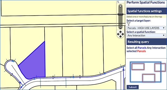
Fig: Spatial Functions Popup Window

Spatial functions available include:

Touching: The Touching function will select the items from the target layer that share a border with the selected object. This does not include items within the object or overlapping the selected object.

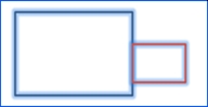
Fig: Touching Spatial Function
Any Interaction: The spatial function Any Interaction will show features with relationships including within, equals, overlapping and touching. The red boxes in the diagram represent the selected map objects.

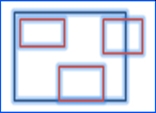
Fig: Any Interaction Spatial Function
Contains: The Contains button is designed to find what the selected feature lies within. The red box in the diagram represents the selected feature.

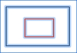
Fig: Contains Spatial Functions
Overlapping: The Overlapping spatial function will highlight the selected target layer that overlaps the selected item on the map.

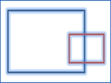
Fig: Overlapping Spatial Functions
Equals: The Equals spatial function can be used to find duplicate items on separate layers.

Fig: Equals Spatial Functions
Inside: The Inside spatial function will highlight the information inside the item selected on the map from the layer chosen in the ‘select target layer’ drop-down box. The red box represents the item selected on the map.

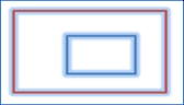
Fig: Inside Spatial Function
Outside: The Outside spatial function is used to find all items outside the selected item on the layer defined in the select a target layer drop-down box. If few objects are selected this tool takes some time to run.

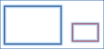
Fig: Outside Spatial Function

Note: The results of a spatial query can be viewed and saved using the Selections Tool.

Spatial Summary

The Spatial Summary tool, located on the Advanced toolbar, displays a polygon summary and a line summary in the Spatial Summary pane. The polygon summary includes the number of polygons selected, the total area and the sum of perimeters. The line summary includes the number of lines selected and the total length of the lines.

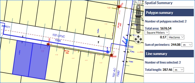
Fig: Spatial Summary Side Pane

Custom Query Builder

The Custom Query Builder tool provides a mechanism to filter features on a layer by specifying criteria based on the feature properties. The user also has the option to apply a spatial Rectangle or Polygon filter to specify the geographical extents on the map to apply to the query. From the resultant list, the user can select an object to zoom to or to add to a selection set.

To setup a basic custom query on land parcels where the parcel area is less than 700m2, and to apply a spatial filter, follow these steps:

The user has the option to set the following parameters:

Layer: The name of the Layer that contains the features to which the query will be applied to selected from a drop-down list.
Property Filter If the tick-box is checked, the subsequent property filters will be applied to the query.
Property: The name of the field to be queried which is selected from a drop-down list based on the Layer selected.
Operator: Pre-defined Operators are available in the drop-down list i.e., Equal to, or Greater than etc.
Value: User entered value which is used to match the property and operator set.
Spatial Filter tick-box: Applies a user defined spatial filter.
Digitize: Allows the user to trace either a Polygon or Rectangle shape on the map to use as the spatial filter.
Output property: Defines which field is displayed in the results window.
Execute: Executes to query defined.
Max results: Sets the maximum number of records returned to the results window.
Scale: Sets the scale for the Zoom to feature option.
Zoom: Zooms to the extents of the feature selected in the results window.

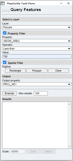
Fig: Custom Query Builder parameters

To setup a basic custom query on land parcels where the parcel area is less than 700m2, and to apply a spatial filter, follow these steps:

Select the Custom Query Builder icon from the Advanced Toolbar. The Query Features pane is displayed.
Select a Layer from the drop-down list to apply the query to.
Check the tick-box next to property to enable the Properties to apply to the query.
Select the Property to use for the filter, for example GEOM_AREA.
Select the Operator to apply to the filter from the drop-down list, for example Less than.
Enter the Value to apply to the filter, for example 700.
Tick the check-box next to Spatial Filter where the user is prompted to draw the extents of the spatial filter on the map. Double-click on the map to complete drawing the Spatial Filter object.

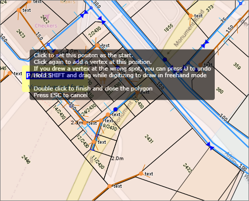
Fig: Custom Query Spatial Filter
Select the Property to display in the resultant list which uniquely describes the feature, for example PRCL_KEY.
Set the Maximum number of results to return to the resultant list, for example 15.
When all query criteria have been entered, select the Execute button.
The results are displayed in the Results window.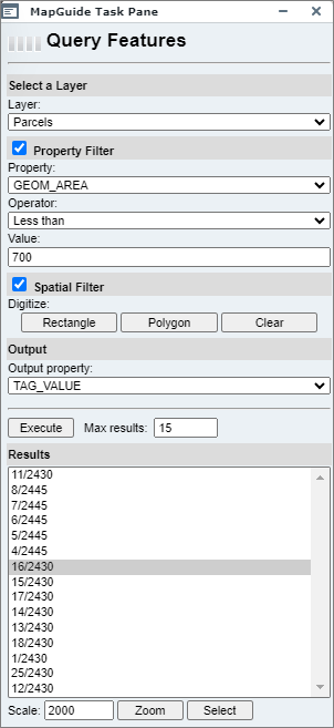

Fig: Custom Query Builder criteria and results
The user can select one of the records in the Results window so that it is highlighted, and select the Zoom button to zoom to the extents of the feature at the scale specified in the Scale text box, for example: 1:2000.
The user can also select one of the records in the Results window and press the Select button to select the feature which can be viewed in Basic Info or Show Info panes.

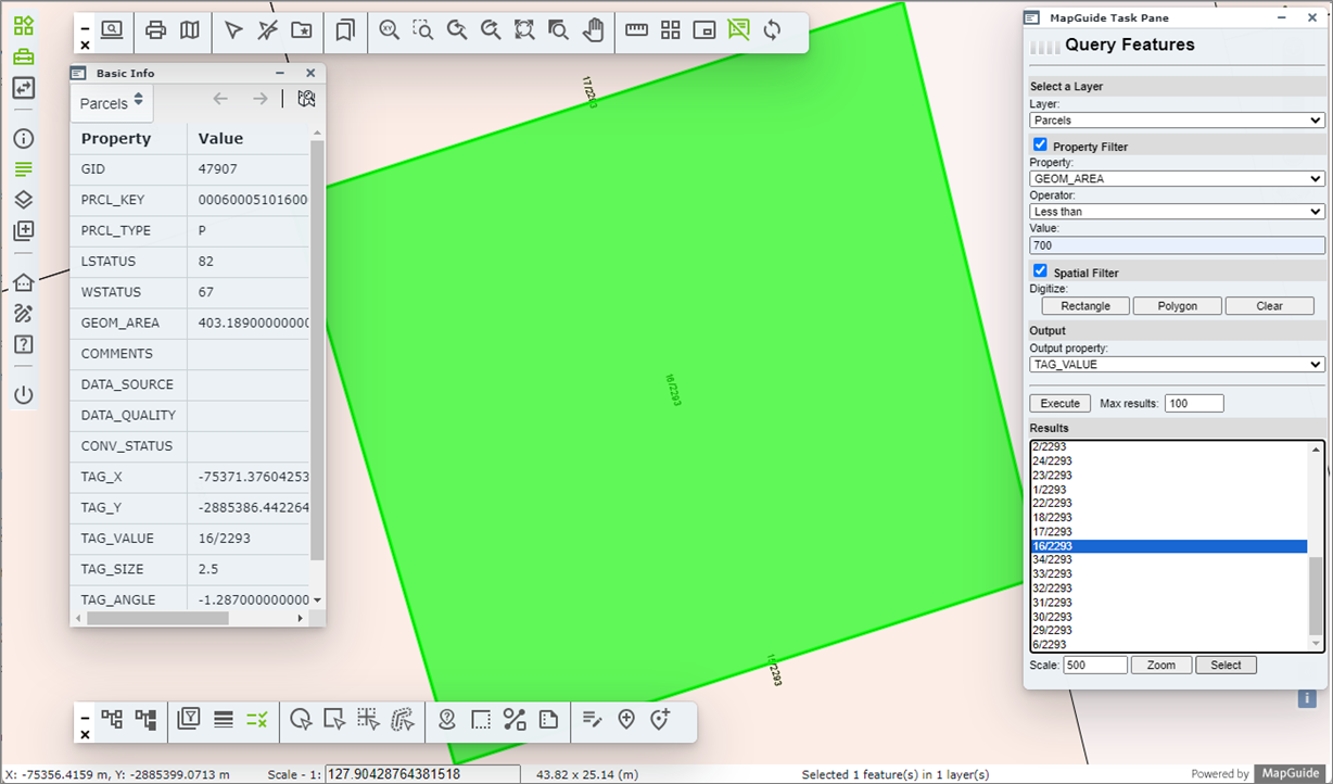
Fig: Select record from Query Results to view in Basic Info or Show Info panes

Geo-scan Images

The Munsys Geo-scan Tools provides Munsys users with a set of functions to capture previously scanned images, for example Engineering as-constructed survey plans, PDF's and DWG files as part of the Munsys data model. This is done in the AutoCAD environment using Spatial Data Manager, where the various functions have been added to the Capture and Change menus. These menu functions allow users to insert, align, scale, and rotate the As-Constructed image/PDF/DWG files so that they are in the correct geographic location to be used as underlying references to capture the spatial location of asset information, and use the markups on the plans to capture required attribute information.

Open Spatial’s enlighten web application enables users to load and display Munsys Geo-scan images as geo-located underlays within the enlighten web browser map. Only one image can be loaded at a time, so if there is already an image loaded, and the user selects another image to load, the newly selected image replaces the previous displayed image.

There are some additional steps required to convert scanned TIF/JPG/JPEG/PDF files to GeoTIFF images which geo-references the image to the correct geographical location with the required scale and rotation angle so that the asset information on other configure enlighten layers can be displayed on top of the Geo-scan image. The conversion process is covered in the FAQ section of the Open Spatial Website.

Note: GeoTIFF is a public domain metadata standard which allows geo-referencing information to be embedded within a TIFF file. GeoTIFF is format extension for storing geo-reference and geo-coding information in a TIFF 6.0 compliant raster file by tying a raster image to a known model space or map projection.

Note: GeoTIFF images may not contain a pound (#) character in the file name since the pound character is reserved exclusively in URLs for use as an anchor. Ensure all pound characters in the image file name are removed to enable the Geo-scan image to load successfully.

View Geo-scan Image Boundary

The Geo-scan boundaries are stored in the spatial table SP_GEOSCAN_BNDRY and can be authored as a layer in enlighten to display the extents of the coverage of the Engineers scanned image. These layers can be authored based on coverage size, or categories assigned to the images based on the utility information appearing in the image, or any other spatial or attribute criteria. For the purposes of the examples below, the layers have been authored based on the coverage extent of the Geo-scan images.

The user can select objects located at a specific location, such as a street intersection, and views the list Geo-scan images which intersect that intersection on the Show Info pane based on the selection set and which layers are switched on for display. The original scanned image can be viewed using the hyperlink setup on Show Info and can also view the scanned image which has been geographically referenced, scaled, and rotated in Munsys. The Geo-scan layer is inserted just above the topmost raster or tile-set layer for display purposes so that all utility layers can be viewed on top of Geo-scan layer.

This enables the capture, integration, and use of scanned Engineering plan images for utility asset inventory recording and other applications. By having the ability to display these scanned plans as back drop images, it improves work efficiency and provides a way to determine which source documents cover a specific geographic area all within a single web browser application. It also provides an electronic filing system where Engineering As-Constructed scanned images can be easily retrieved and viewed from the central server from a single source.

Note: The Geo-scan image layer is displayed above the other base layers so that any utility data layers can be displayed on top of the Geo-scan image.

Load Geo-scan Images

The geo-scan boundary is used as a geo-referenced frame for the as-constructed image to enable the users to identify the physical location of the as-constructed plan. The geo-scan image can then be loaded into the frame at the positioned scale and rotation to provide a backdrop of the captured utility assets such as pipes and nodes. The Geo-scan image layer should be authored to display below all other layers so that parcel and utility data can be viewed on top of the geo-scan image when loaded.

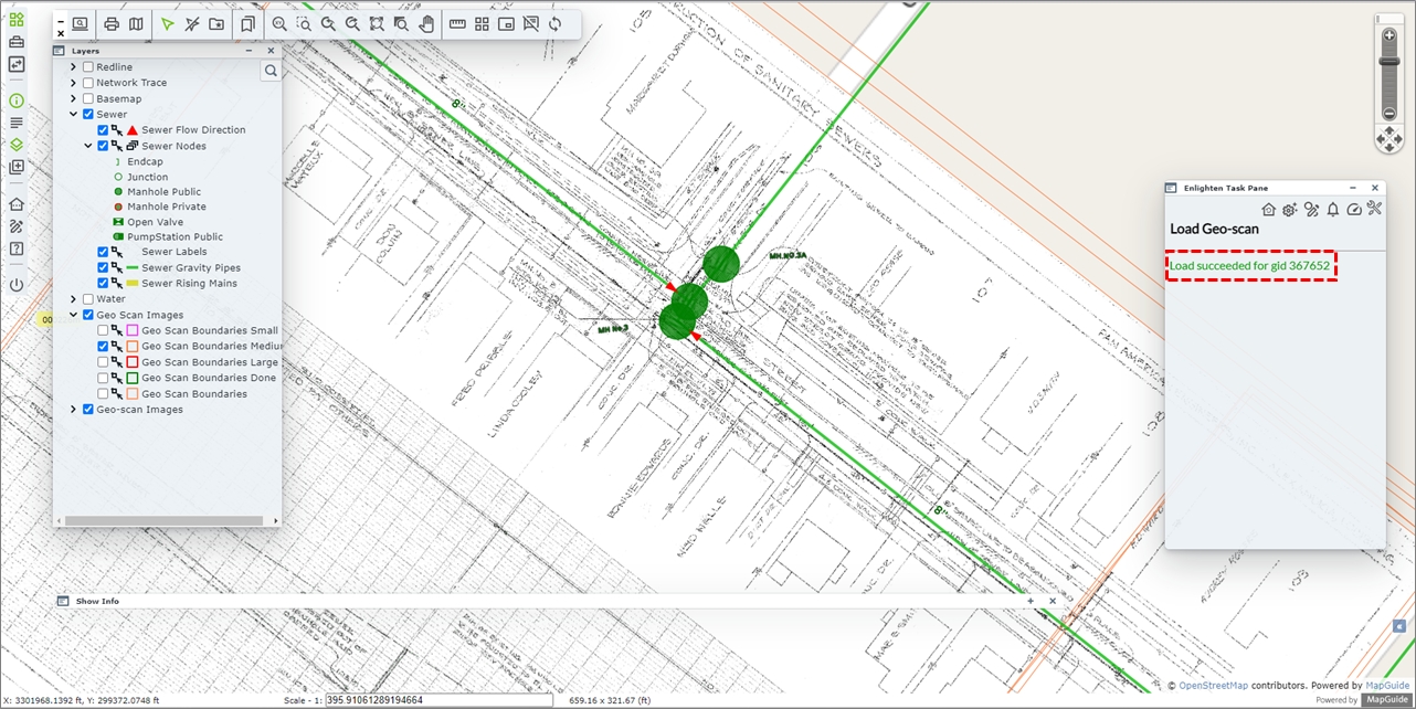
Fig: Utility data is displayed on top of the As-Constructed Image

To Load a Geo-scan image, follow these steps:

Zoom to the specified location on the map and switch on the required map layers to display utility information such as the sanitary sewer pipes as well as the Geo-scan boundary layer/s. This will differ for each customer depending on how the geo-scan boundary layer is authored on setup.
Select all objects on the map around the road intersection of interest to be displayed in the Show Info pane. Only map objects on displayed layers can be selected.

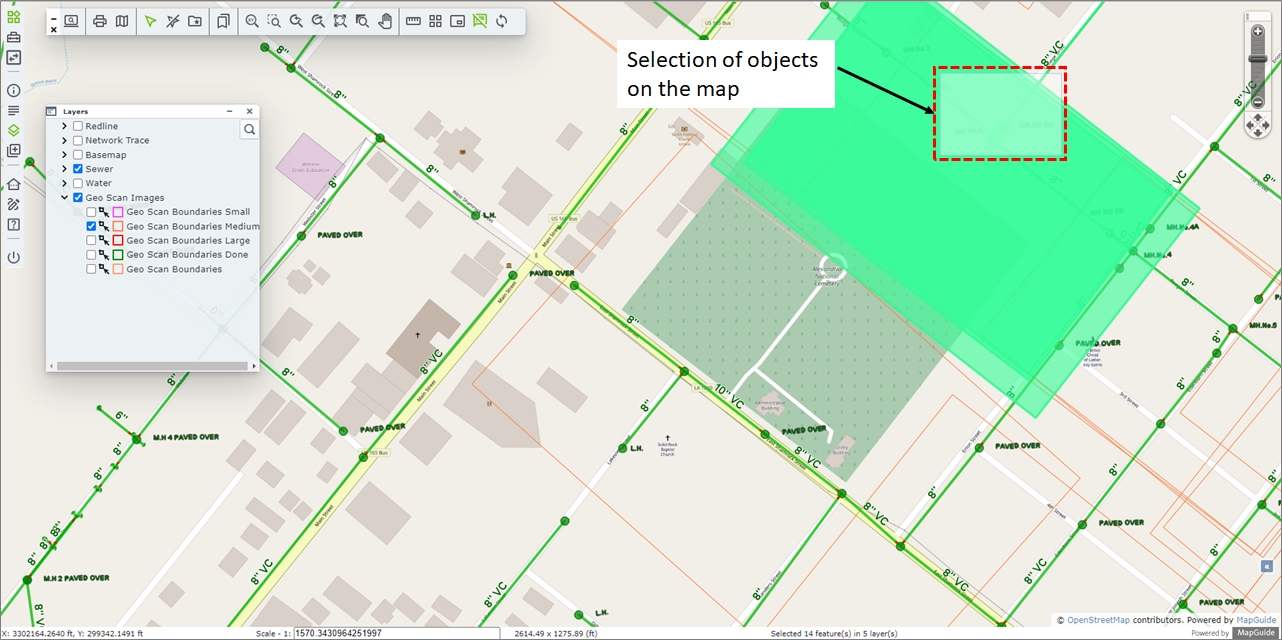
Fig: Selection of Geo-scan boundary objects crossing a specific street intersection
Select the Show Info icon on the Main toolbar which opens the Show Info pane and populates the pane with the attribute information for the objects selected where Show Info Forms have be configured. Those objects displayed in grey in the Tree View do not have any Show Info forms configured.
If the Show Info form for Geo-scan boundaries is setup to display the Image Preview for URL type columns, as soon as the Geo-scan layer is selected the Image Preview window is displayed on top of the Show Info pane for the first record displayed in the List View.

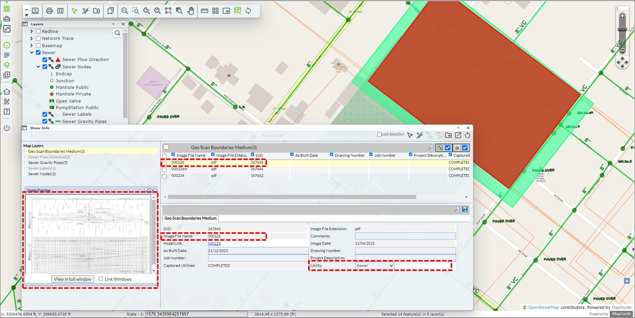
Fig: Select the Geo-scan hyperlink on the Advanced Form
Navigating through the records in the List View updates the corresponding attributes in the Detail View as well as the Image Preview window.

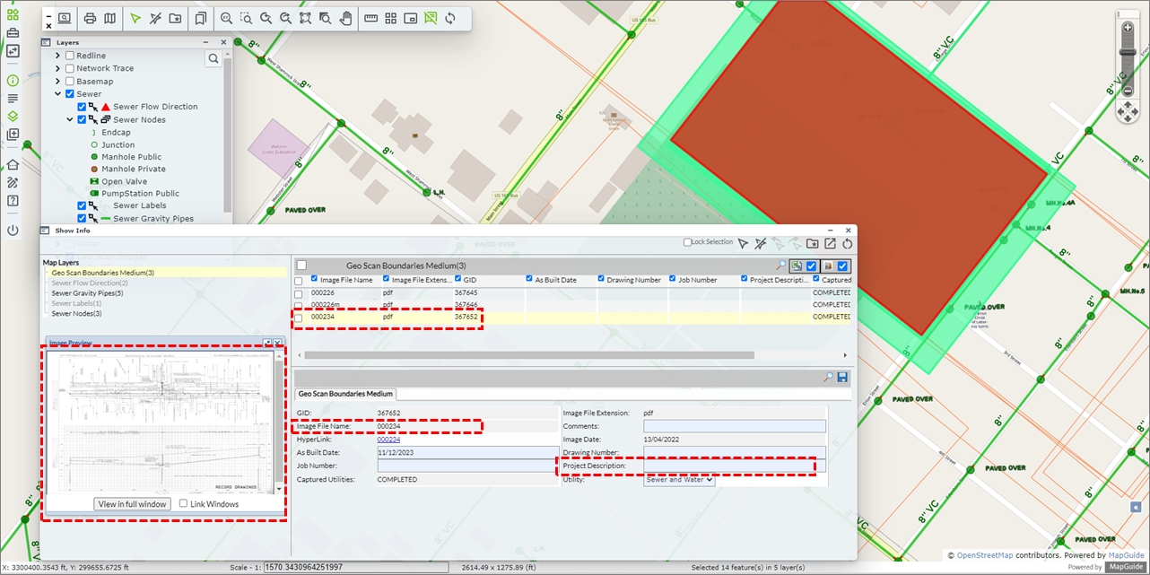
Fig: Select the Geo-scan hyperlink on the Advanced Form
Selecting the option View in full window loads the geo-scan image in a separate browser window in the format it was scanned, either TIF/JPG/PDF, where you can then zoom in and navigate around the scanned image to pick up critical information and notations.

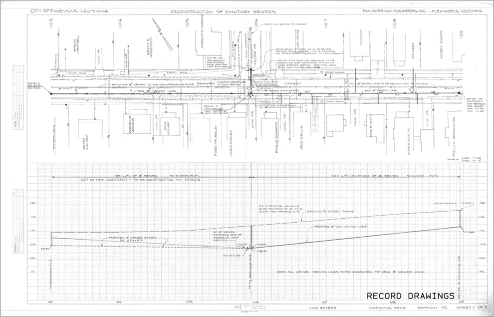
Fig: Viewing Original Geo-scan Image
The user can close the Image Preview window by selecting the Close button , or minimize by selecting the Minimize button in top right-hand corner of the Image Preview window.
By selecting a single Geo-scan record in the list view on the Show Info pane, you can then navigate to the selected record in the map by selecting the Zoom to Map icon. The map will display zoom to the extents of the selected Geo-scan boundary and the selection set is updated to the single record in the Show Info pane.

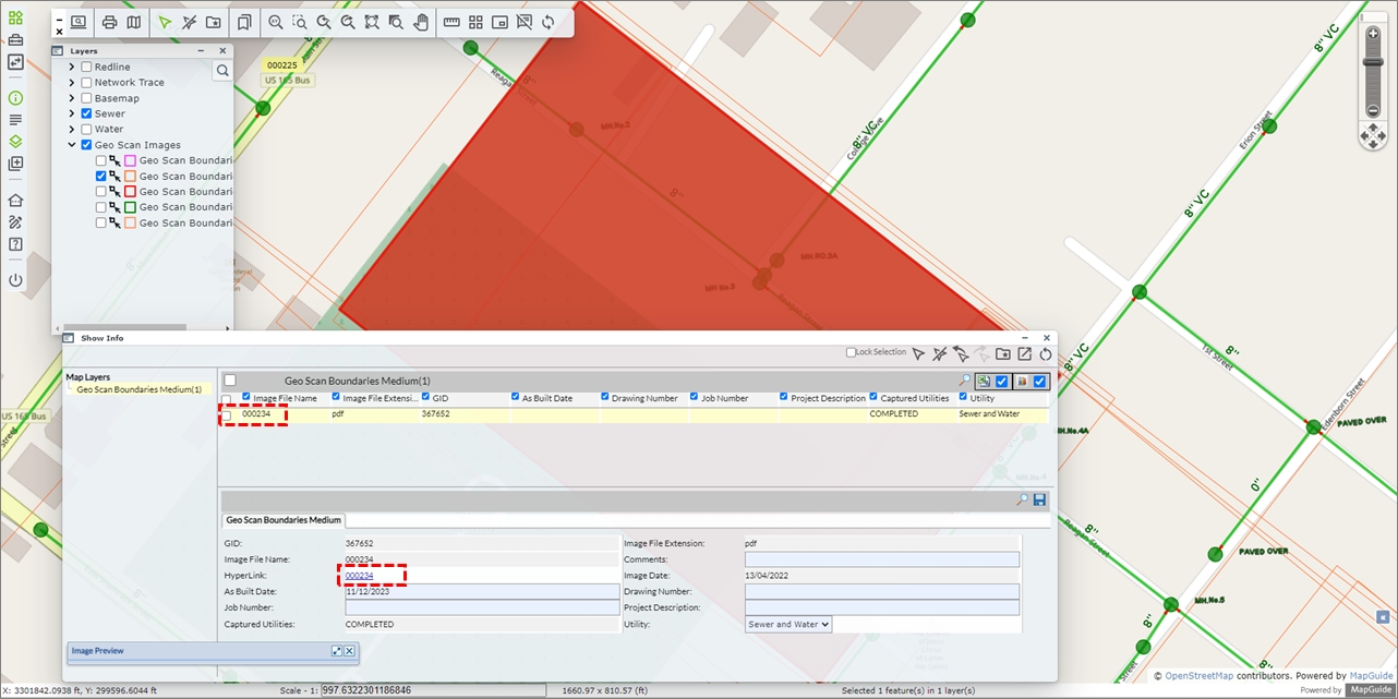
Fig: Selecting single record to Zoom to Map
On the map, right-click on the highlighted geo-scan boundary and select the Load Geo Scan icon from the context menu to load the geo-referenced image as a back-drop on the Geo Scan Image layer.

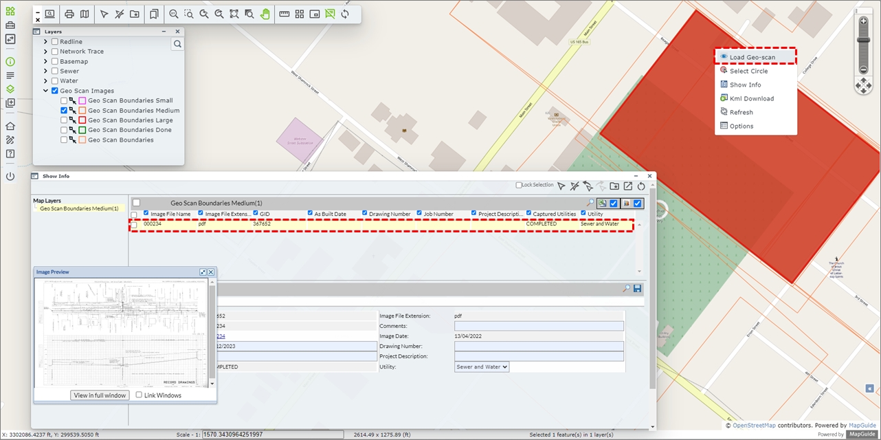
Fig: Load the Geo-scan image from the Context Menu
The Geo-scan layer is inserted just above the topmost raster or tile-set layer for display purposes so that utility layers can be viewed on top of Geo-scan layer and a message is displayed indicating the image has been successfully loaded.

Fig: Load the Geo-scan image from the Context Menu
You can zoom in and out of the map while navigating around the scanned As-Constructed Engineering image to check that what has been captured in the GIS spatial tables matches what was constructed in the field.

Managing Geo-scan Error Messages

All Geo-scan images should be stored in a separate folder on the MapGuide server or on a shared folder location on the network so that the file path location stored with the geo-scan image in the database corresponds to the file location on the server.

All geo-scan image boundaries and the associated geo-scan image are stored in the spatial table SP_GEOSCAN_BNDRY. The list of columns below will assist the GIS Administrator to troubleshoot the error messages when the geo-scan images fail to load.

COLUMN NAME	DESCRIPTION
IMG_FILEPATH	Stores the file path location or shared folder location for each geo-scan image, for example: *C:\websites\Pineville5\Data\Pdf_Files\PADDED\*
IMG_FILENAME	Stores the file name of the geo-scan image, for example: *533881*
IMG_FILEEXT	Stores the file type extension, for example: *tif*

Should a Geo-scan image fail to load in the map, an error message is displayed in the Enlighten Task pane indicting the name and location of the file being referenced in the URL for the selected Geo-scan Boundary. Refer the error message to your Administrator to check that the file exists on the enlighten server in the specified folder location.

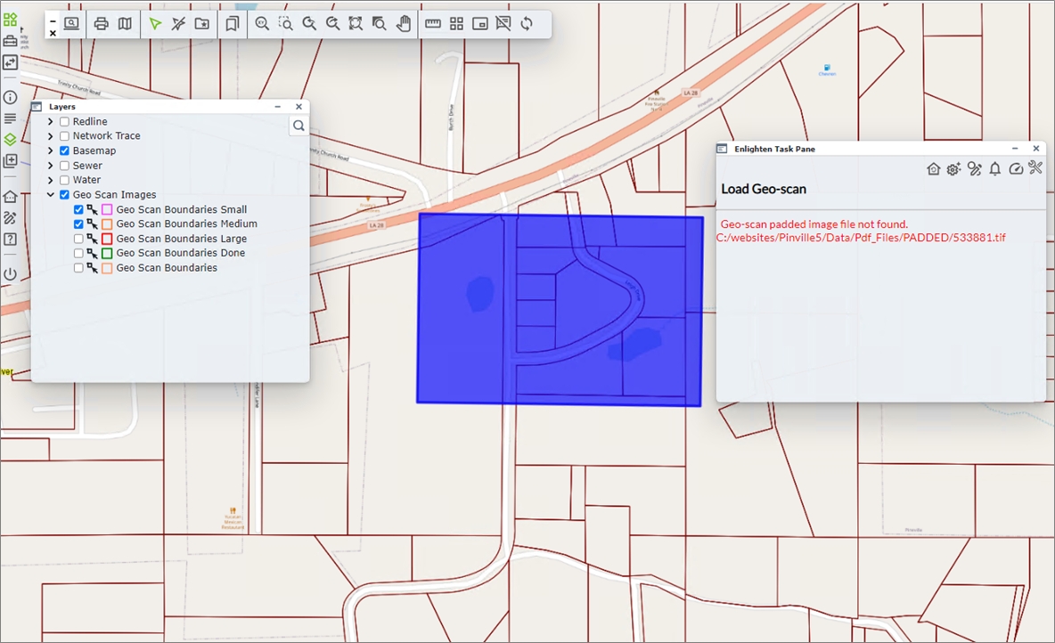
Fig: Geo-scan Image failed to load
In the event geo-scan images cannot be located when previewed in the Show Info pane, or the image file extension type does not match what is stored in the database, an error message is displayed in the preview pane indicating that the selected geo-scan image is either invalid or cannot be found in the file path / file name columns stored in the database.

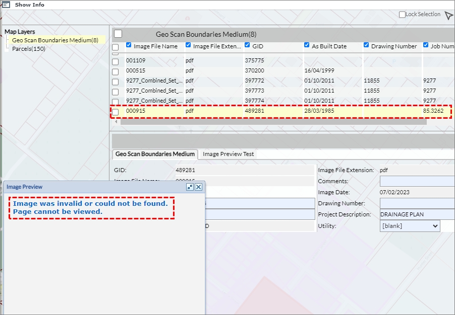
Fig: Geo-scan Preview Image error message